In this post we'll explore how to use a machine learning model to append predictions to a Fabric data lake table.

In this scenario, our Data Scientist has already trained and registered a predictive machine learning model with Fabric using the Fabric Data Science workload.

The Predictive Model

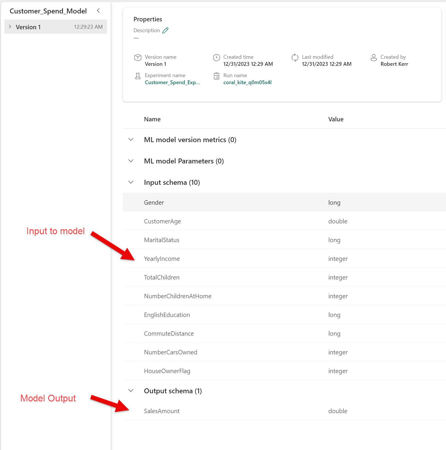
The model is registered in our Fabric Workspace with the name Customer_Spend_Model. Reviewing the image below, we can see the model takes as input a list of customer demographics--such as CustomerAge and YearlyIncome. In all there are 10 demographic features used as input to the model.

The predictive model was trained on a set of approximately 9,000 current customers with known lifetime sales volume. When a new customer's demographics are fed to the model's Input schema, the model will predict the future SalesAmount for the new customer as the only field in the Output schema.

The ML Model registerd with Fabric's MLflow catalog

The Input Table

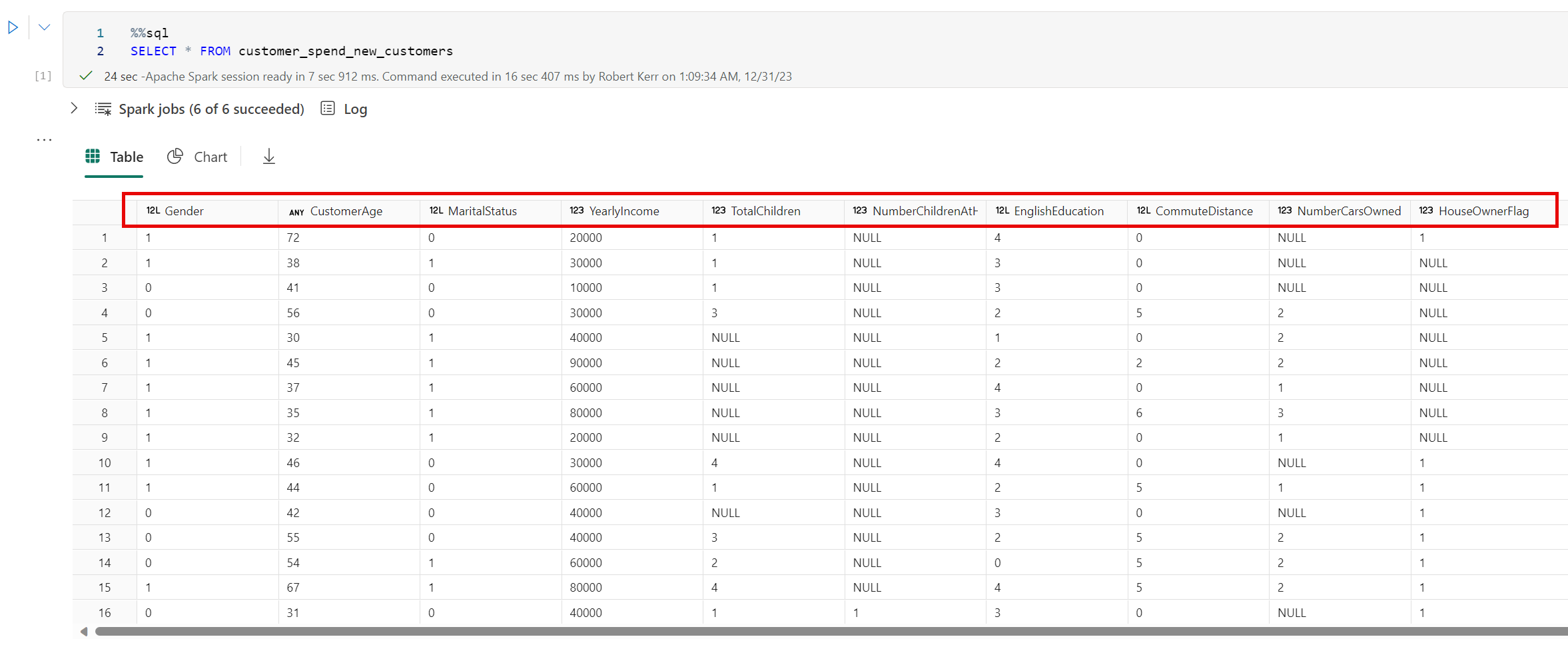
In this example, we've received a set of 100 new customers, and stored them as a Delta table in Fabric. A subset of the input table is below.

💡

Note that the table contains columns that exactly match the Input schema of the Customer_Spend_Model.

The input table illustrated below doesn't include a column for SalesAmount. These are new customers, and we'll use the model to predict what the lifetime value of these new customers will be based on what we know of past customers.

💡

The end result of this process is to append a new column to the data frame that contains a predicted sales amount.

Using the Fabric PREDICT function

While we could write code to iterate over the table and predict each row's value, in the Fabric data lake environment there's an easier way.

Fabric provides an MLFlowTransformer class that can be used to automatically load a ML model stored in the Fabric Model Registry (which is MLflow-based) and apply the model to each of the rows in a PySpark DataFrame. The effect is to append the model's Output schema to each row.

Load the Input Data

We'll use the contents of the customer_spend_new_customers table pictured above as the input data. All we need to do is read the input table into a PySpark DataFrame. I'll use SQL to read the data, though using the Python syntax would work just as well.

df = spark.sql("SELECT * FROM customer_spend_new_customers")

Reading the input table from the Data Lake

Run the Input Data Through the Transformation

To create a new DataFrame consisting of the original DataFrame with ML Model output appended, we can use the following code:

# Import the transformer 
from synapse.ml.predict import MLFlowTransformer

# Create a transformer instance, providing the model name and input/output column names
model = MLFlowTransformer(
    inputCols=df.columns,
    outputCol='PredictedSales', 
    modelName='Customer_Spend_Model'
)

# Process the input DataFrame by appending a prediction column
df_output = model.transform(df)

Code to append prediction column to the data frame

Save the Transformed DataFrame as a Delta Table

Finally, we'll save the new DataFrame--with the sales prediction appended--back to the Data Lake as a Delta table.

# Write the DataFrame to a Data Lake table
df_output.write \
  .format('delta') \
  .mode("overwrite") \
  .saveAsTable('Customer_Spend_Predictions')

Code to save the output DataFrame to the Data Lake as a Delta table

Review the Sales Predictions

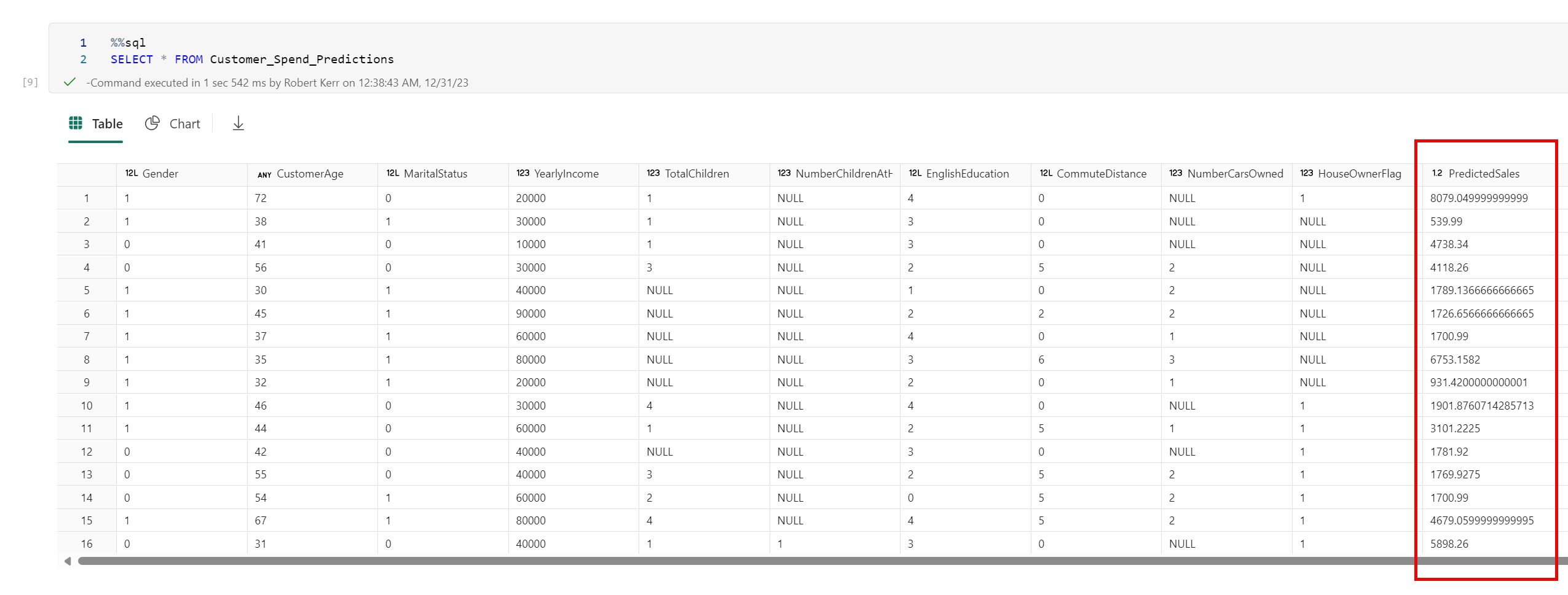
Now that the table is saved to the Data Lake as a Delta table, it becomes part of the semantic model, and is accessible from PySpark, the SQL endpoint and from Power BI.

Note the new Delta table has all the columns of the original--and one additional column with predicted sales.