


In this post I'm, going to walk through step-by-step how to connect a single Jupyter notebook to two Lakehouses, and then easily read & write data between them. In a medallion architecture, we can process data between Bronze/Silver/Gold Lakehouses using Data Flows, Data Pipelines or Notebooks. In this example I'll use a notebook.
Initial Configuration
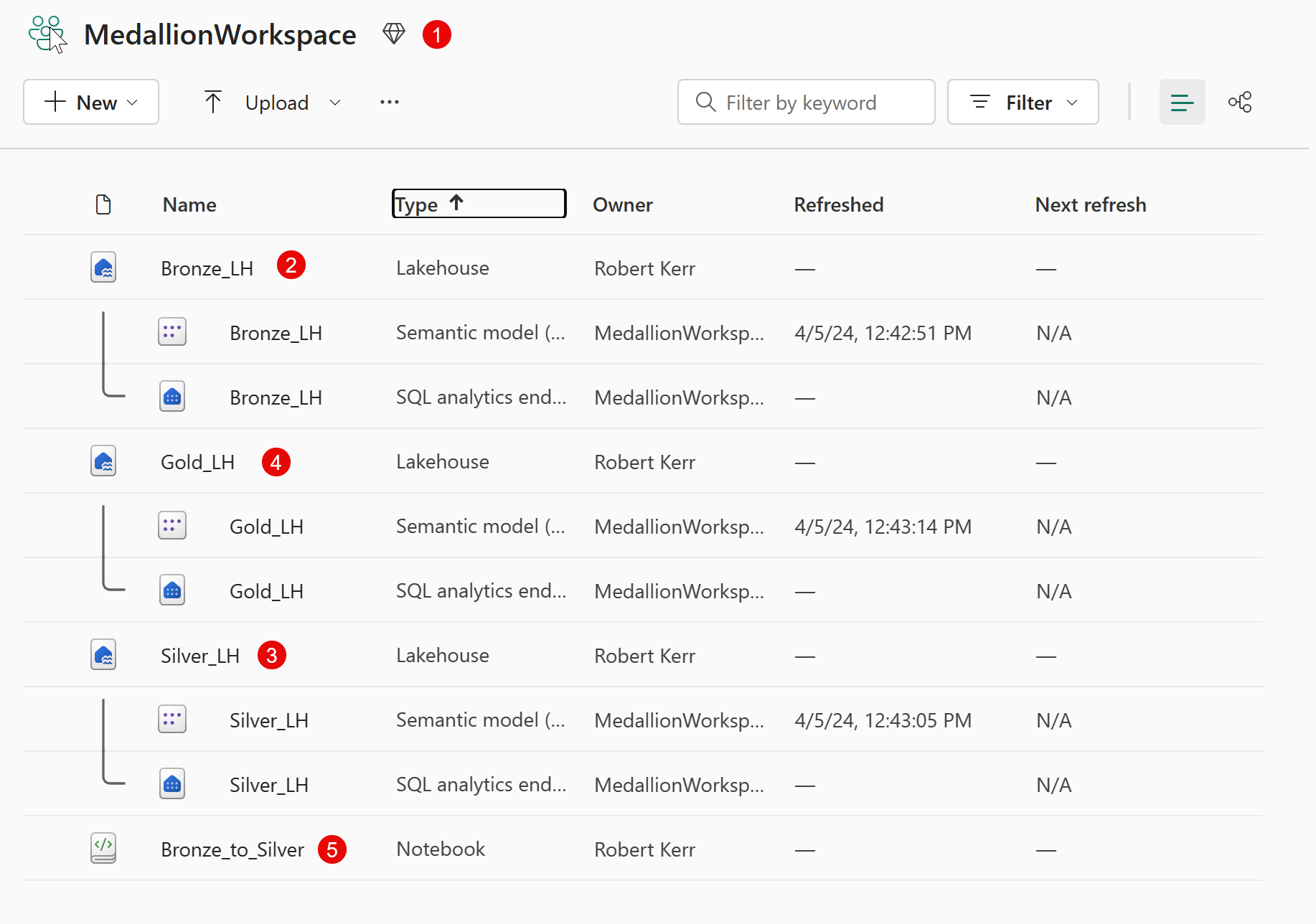
To start, I have the following artifacts in my solution:
- Workspace named
MedallionWorkspace, that contains my entire solution. - Lakehouse named
Bronze_LH - Lakehouse named
Silver_LH - Lakehouse named
Gold_LH - Jupyter Notebook named
Bronze_to_Silverwhere I'll conduct my data import (from Bronze), processing, and output (to Silver).
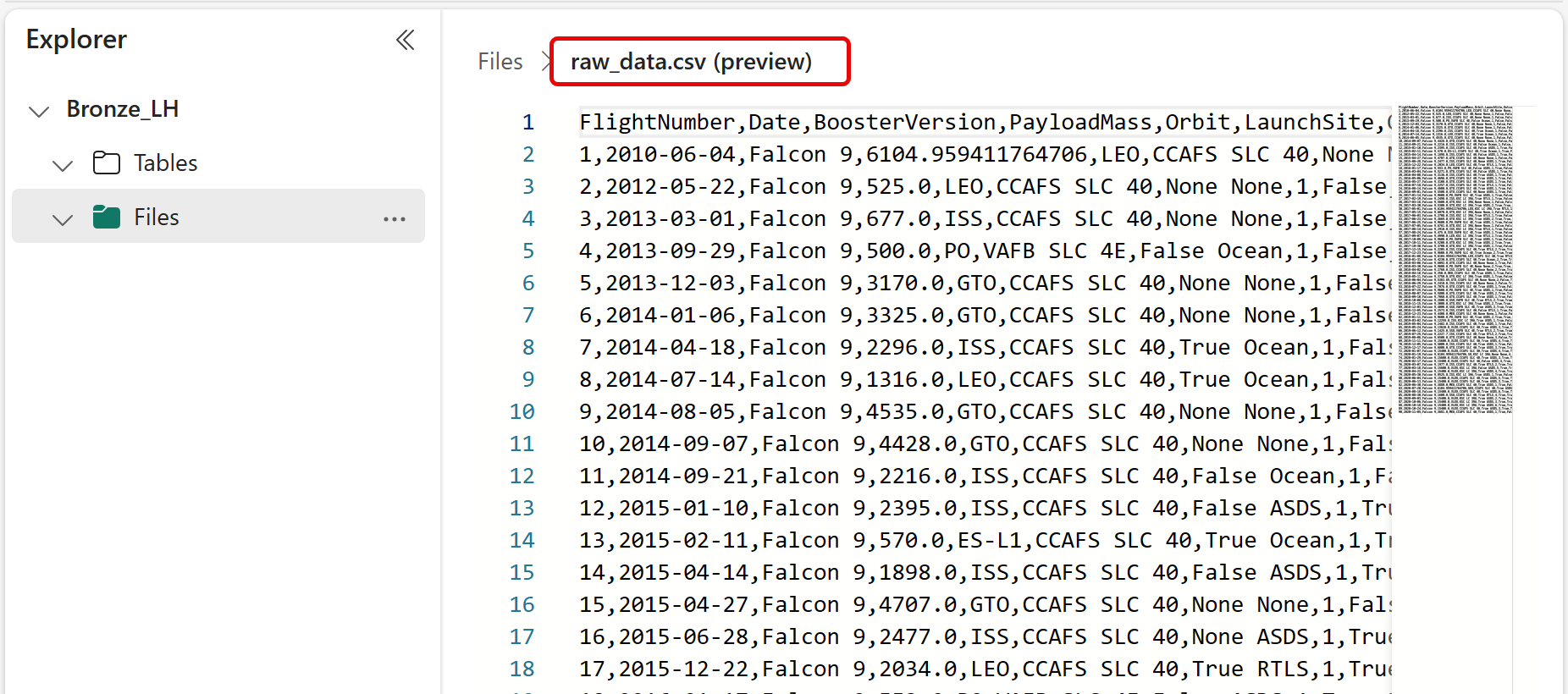
Within the Bronze Lakehouse I have an input file named raw_data.csv. In this post, I'm going to:
- Read the input CSV file from
Bronze/Files into aDataframe. - Transform the Dataframe by adding a current date/time column.
- Write the Dataframe as a CSV back to the original
Bronze/Files folder. - Write the Dataframe as a CSV to
Silver/Files. - Write the Dataframe as a Delta table to
Bronze/Tables. - Write the Dataframe as a Delta table to
Silver/Tables.
Add Bronze and Silver Lakehouses to the Notebook
Since we'll be referencing both Lakehouses when reading the CSV and writing Tables, we'll first add both Lakehouses to the explorer navigation tree of the Notebook.
Click the Add button to get started.
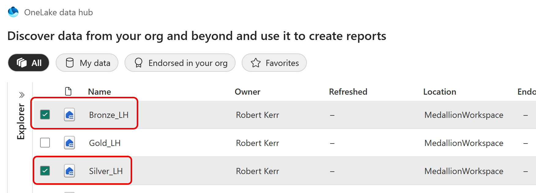
Select Bronze and Silver Lakehouses. We don't need to select Gold because we're not going to access that data in this Notebook.
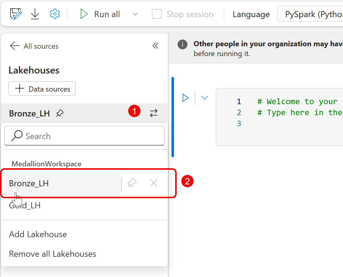
Next, in the sidebar, select the Bronze Lakehouse as the current context.
Read the Data File from Bronze
In the first cell, let's just read the source CSV file into a Dataframe. Because the source data is in Bronze, and that's the default Lakehouse, no special syntax is needed yet.
df = spark.read.format("csv") \
    .option("header","true") \
    .load("Files/raw_data.csv")
Transform the Dataframe
To show that we can process the data, let's add a new column to the Dataframe. This column will simply state the date/time the data processing occurred.
from pyspark.sql.functions import current_timestamp
df = df.withColumn("processed_date_time", current_timestamp())
Write the Data back to Bronze
Writing the Dataframe back to Bronze is trivial and requires no special syntax. Here we'll write it both as a CSV to the Files section, then as a Delta table to the Tables section.
# Write a CSV file
df.write.mode('overwrite') \
    .csv('Files/output_csv_Bronze.csv')

# Write a Delta Parquet table
df.write.format("delta").mode("overwrite") \
    .saveAsTable('output_table_Bronze')
Write the Data to Silver
Now, let's do the same thing, but to Silver. In this case, since Silver is not the current Lakehouse context, we need to use some additional syntax sugar:
- For the Files section, we'll use the
mssparkutilslibrary to mount theSilver_LHLakehouse in the context of the notebook. - For the Tables section, it's easier--we can just use a two-part reference to access tables in any Lakehouse that's connected in the notebook, but not the current Lakehouse.
First, let's create a function that will get a mount path given a Lakehouse name.
def get_mount_path(lakehouse_name):
    mnt_point = f'/mnt/mnt_{lakehouse_name}'
    mssparkutils.fs.mount(lakehouse_name, mnt_point)
    return f'file:{mssparkutils.fs.getMountPath(mnt_point)}'
Next, let's write the CSV file to Silver_LH/Files, using the function defined above in-line to build a full URL for the output table.
mount_path = get_mount_path('Silver_LH')

df.write.mode('overwrite') \
    .csv(f'{mount_path}/Files/output_csv_Silver.csv')
And finally, we'll write the Dataframe as a Delta Parquet table in Silver. This time the change is trivial, just adding Silver_LH. to the beginning of the output table name.
df.write.format("delta").mode("overwrite") \
    .saveAsTable('Silver_LH.output_table_Silver')
Summary
And that's it for this post. While it's not entirely obvious how to reference multiple Lakehouses in a Notebook, it's fairly straightforward once you know the syntax!